Supervised Classification

In this section we introduce the classification problem, work with some initial examples, and describe the training and testing phases involved in creating a classifier. We also take a first look at validation and overfitting. By the end of this section, you should be able to:

• Describe the classification problem

• Describe at a high level the linear classifier and the perceptron algorithm

• Describe the training and testing phases

• Plot and interpret a decision boundary and decision matrix to understand model performance

Introduction

Classification is the problem of predicting a dependent variable that takes values from a finite, discrete set. An ML model that predicts such a dependent variable is called a classifier. The possible values are called classes.

An important special case is a binary classifier which predicts a dependent variable which takes on just two possible values. That is, a binary classifier is a model which predicts two classes for the dependent variable.

For example, given the cellular features of a biopsy, a physician might want to predict if a tumor is benign or malignant. The dependent variable here is whether or not the tumor is malignant. There are two possible values:

• Benign

• Malignant

These are the two classes of the dependent variable, and an ML model that predicts this variable will thus be called a binary classifier.

Consider the following dataset depicting cell nuclei features from histology images and prognosis.

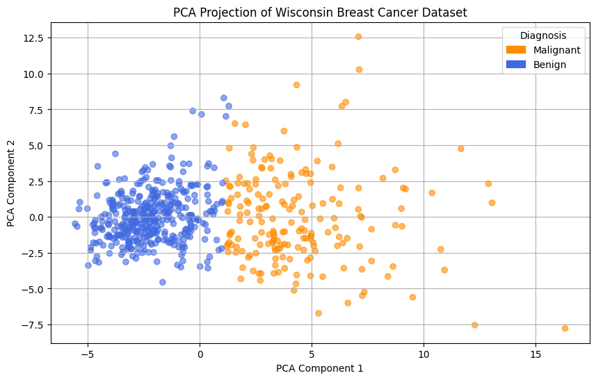
Sample data showing principal component analysis on cell nuclei features and tumor classification as benign or malignant.

We can use this data to build an ML model for predicting whether an individual’s tumor is benign or malignant. The process is as follows:

1. Collect and prepare data about nuclei size, shape, and texture.

2. Train a model using some of the prepared data.

3. Validate the model using some of the prepared data.

4. Deploy the model to predict tumor classification for new individuals.

How might we train a classifier? There are many techniques. The first one we will look at is called linear classification. Before we look at some of the details of linear classification, does anyone have an intuition about how one might proceed to determine which tumors are malignant?

Is the image above suggestive of a way to predict the tumor type?

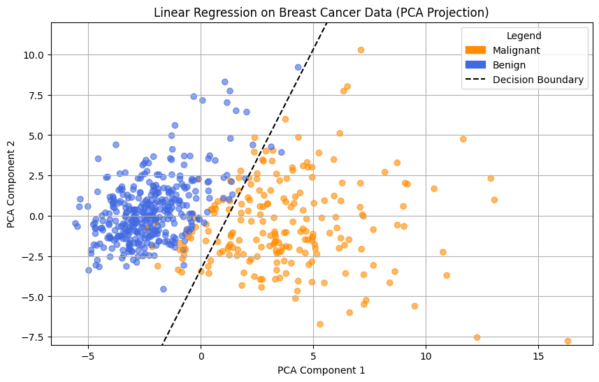
A linear decision boundary. Data points are classified based on which side of the line they fall.

One approach is to use a linear equation (i.e., a line) to determine which class a data point belongs to. In the picture above we have drawn one possible line. Points on the left side of the line are classified as “benign” and points on the right are classified as “malignant”.

Linear Classification with Scikit Learn

Let’s implement a linear classifier using the sklearn package. In this first example, we’ll illustrate the techniques on a classic dataset that describes iris flowers. We’ll also introduce helper functions for splitting data into a training data and testing data and computing the accurary of our trained models.

First, let us begin with a description of our dataset. The Iris Flower Dataset or Fisher’s Iris Dataset was published in a paper by British biologist Ronald Fisher in the paper, The use of multiple measurements in taxonomic problems (see [2]). The dataset includes four features for 150 samples of three species of iris: setosa, virginica, and versicolor. The features are: sepal length, sepal width, petal length, and petal width, all measured in cm.

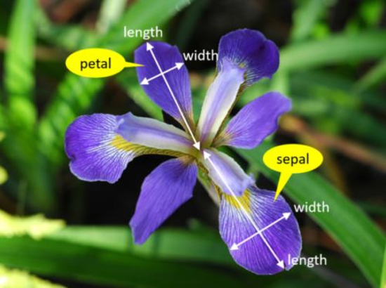
Diagram illustrating sepal and petal length and width, adapted from De Silva, 2020.

Loading the Data

First, let us begin by loading the dataset. We’ll use a Jupyter notebook for this portion since we will want to make use of some visualization.

The sklearn package provides a convenience method for loading several classical datasets, including the Iris Flower Dataset:

>>> from sklearn import datasets
>>> iris = datasets.load_iris()

As mentioned, this dataset contains 4 features for 150 samples of three different species of iris. Like all datasets objects from sklearn, the iris object contains a data attribute holding the independent variables as well as a target attribute containing the dependent variable for each sample. Each attribute is a numpy.ndarray. There are also attributes features_names and target_names which contain the names of the independent and dependent variables, respectively.

We can explore the dataset with Python:

>>> iris.feature_names
['sepal length (cm)',
'sepal width (cm)',
'petal length (cm)',
'petal width (cm)']

>>> iris.data
array([[5.1, 3.5, 1.4, 0.2],
     [4.9, 3. , 1.4, 0.2],
     [4.7, 3.2, 1.3, 0.2],
     [4.6, 3.1, 1.5, 0.2],
     [5. , 3.6, 1.4, 0.2],
     . . .

>>> type(iris.data)
<class 'numpy.ndarray'>

>>> iris.target_names
array(['setosa', 'versicolor', 'virginica'], dtype='<U10')

>>> iris.target
array([0, 0, 0, 0, 0, 0, 0, 0, 0, 0, 0, 0, 0, 0, 0, 0, 0, 0, 0, 0, 0, 0,
     0, 0, 0, 0, 0, 0, 0, 0, 0, 0, 0, 0, 0, 0, 0, 0, 0, 0, 0, 0, 0, 0,
     0, 0, 0, 0, 0, 0, 1, 1, 1, 1, 1, 1, 1, 1, 1, 1, 1, 1, 1, 1, 1, 1,
     1, 1, 1, 1, 1, 1, 1, 1, 1, 1, 1, 1, 1, 1, 1, 1, 1, 1, 1, 1, 1, 1,
     1, 1, 1, 1, 1, 1, 1, 1, 1, 1, 1, 1, 2, 2, 2, 2, 2, 2, 2, 2, 2, 2,
     2, 2, 2, 2, 2, 2, 2, 2, 2, 2, 2, 2, 2, 2, 2, 2, 2, 2, 2, 2, 2, 2,
     2, 2, 2, 2, 2, 2, 2, 2, 2, 2, 2, 2, 2, 2, 2, 2, 2, 2])

>>> type(iris.target)
numpy.ndarray

Notice that the features are encoded as floats and that iris.data is a 2d-array of shape 150x4. Similarly, the target classes are encoded with integers (0, 1, and 2) for the 3 different species, and that iris.target is a 1d-array of shape 150x1.

To simplify our initial discussion, we are going to consider the subset of the data consisting of all samples in the first two classes (0 and 1), and we will also only consider the petal length and petal width features (columns 3 and 4). Notice that the first 100 data points belong to classes 0 and 1 (the last 50 belong to class 2), so we can construct our dataset as follows:

>>> # only use the first 100 rows and the last two columns
>>> X = iris.data[0:100,2:4]

>>> # only use first 100 rows
>>> y = iris.target[0:100]

Note that we have organized the data into the objects X and y for the independent and dependent variables, respectively. This is a common convention we will use throughout the workshop.

Training the Model

Let us take a moment to recall the general strategy for working with ML models.

1. Collect and prepare data with labels.

2. Train a model using some of the prepared data.

3. Validate the model using some of the prepared data.

4. Deploy the model to predict the default status for new individuals.

We have completed step 1 for the iris dataset – we are ready to move to step 2.

We need to use some of the data for training and reserve some for testing how well the trained model performs on data it hasn’t seen. This is a very important aspect of machine learning. If you use data the model has already seen in training to test it, you are undermining the integrity of the test.

In general, we’ll want to train the model using “most” of the data and only hold back a relatively small amount to use as validation. What is “most” and how do we decide what to hold back for testing? There are a lot of aspects to this question, and we will revisit the topic throughout the workshop, but for now, we’ll split the data using 70% for training and 30% for testing.

We’ll also use a “stratification” technique to ensure (as much as possible) that the split preserves proportions of the target class. Fortunately, sklearn has a function to do the work for us.

The train_test_split function from sklearn is very helpful here:

>>> from sklearn.model_selection import train_test_split
>>> X_train, X_test, y_train, y_test = train_test_split(X, y, test_size=0.3, stratify=y, random_state=1)

In the code above, we are collecting 4 new objects: X_train, X_test, y_train, y_test representing a splitting of the X and y data. The 0.3 specifies that we want 30% of the data to be used for test data and 70% to be used for training.

Next, we specify stratify=y. This is a very important parameter. Conceptually, it instructs sklearn to split the data in a way that preserves the frequency of occurrence of different target classes. In our case, we have an equal number of samples for each target (50 each), so a random splitting is likely fine. But in general, using a stratified split will ensure a proportional splitting even when the samples are imbalanced.

Finally, we specify random_state=1. This controls the randomization that is used in a way that guarantees deterministic results. That is, when setting a value for random_state, repreated calls to train_test_split will always result in the same splitting for the same input data. This has important consequences for reproducibility, a topic we will revisit throughout the unit.

Having split the data, we are ready to train our model. We’ll use the SGDClassifier class from the sklearn.linear_model module. The “SGD” stands for “Stochastic Gradient Descent” and the SGDClassifier provides a family of models based on an associated family of Gradient Descent algorithms.

In the code below, we first instantiate the SGDClassifier object, specifying some configurations. Then we actually perform the model training using the fit function.

Naturally, we use the training data when calling fit:

>>> from sklearn.linear_model import SGDClassifier

>>> # the alpha is used for the learning rate, which can impact overfitting vs underfitting,
>>> # something we haven't discussed yet, but just note that a higher value of alpha more likely
>>> # to underfit. Can try changing alpha=0.05 if the model doesn't achieve 100% accuracy.
>>> clf = SGDClassifier(loss="perceptron", alpha=0.01)

>>> clf.fit(X_train, y_train)

Note that we specify loss="perceptron" to indicate we want to use the Perceptron algorithm [1]. The SGDClassifier supports several other algorithms (e.g., “hinge”, “squared_hinge”, “log_loss”, etc.).

The alpha parameter deals with something called regularization, which we haven’t discussed yet – ignore it for now.

The clf object is the trained model, and it can be used to predict the species of iris samples using the clf.predict() method.

Validation

Now that the model has been trained we can proceed to step 3 – validation. Our goal here is to compute the accuracy of our model against the test dataset (i.e., the _test data objects above). We’ll also compute the accuracy of the model against the training data to see how they compare.

For validation, we’ll make use of another helpful function: the accuracy_score from the sklearn.metrics module. The basic usage is straightforward:

>>> from sklearn.metrics import accuracy_score

>>> # Check the accuracy on the test data
>>> accuracy_test=accuracy_score(y_test, clf.predict(X_test))

>>> # Check accuracy on the training data
>>> accuracy_train=accuracy_score(y_train, clf.predict(X_train))

As suggested by the code above, the accuracy_score function takes two parameters: the target (dependent) variables and the predictions on the independent variables. Our dependent variables are just the y_test and y_train objects defined before, and for the prediction, we apply the clf.predict function to each of the X_test and X_train arrays, respectively.

The result returned by accuracy_score is simply a float from 0 to 1 containing the fraction of correctly classified samples.

How did our model do?

>>> accuracy_train
1.0

>>> accuracy_test
1.0

In fact, our model was perfect on both the test and training data! One way to understand this is to visualize the data – the Iris dataset is linearly separable, as we will see.

Additional Properties of the Model

• clf.classes_: These are the possible target class values the model is trying to predict.

• clf.decision_function(): This function computes the actual decision value for a given X that is used by the predict() function. Note that it requires an array of the same shape as the data on which it was trained.

• clf.coef_: The coefficients learned. Note that when the target (dependent variable) is 1-dimensional, as in the case above, the coef_ attribute will be a 1-D array of length equal to the number of features.

• clf.intercept_: The y-intercept learned. Together with clf.coef_, this determines the clf.decision_function.

Examples:

>>> clf.classes_
array([0, 1])

>>> clf.coef_
array([[2.17976136, 0.84768497]])

>>> clf.intercept_
array([-6.61195757])

>>> # consider one data point; it's a 1-D array with two values:
>>> X_train[0]
array([1.5, 0.2])

>>> # apply the decision_function to a single value (note the shape of the input):
>>> clf.decision_function([X_train[0]])
array([-3.17277854])

>>> # this is the same as computing the linear combination of the coef_ and intercept_:
>>> import numpy as np
>>> np.sum(clf.coef_*X_train[0]) + clf.intercept_
array([-3.17277854])

>>> clf.decision_function(X_train)
array([-3.17277854,  4.46849599, -3.08801005, -3.39075468, -3.60873082,
   -4.12945158,  4.51693513, -3.17277854,  5.37672989, -3.00324155,
   . . .

>>> # note that class predictions agree with the assoicated sign (positive or negative) of
>>> # the decision_function above
>>> clf.predict(X_train)
array([0, 1, 0, 0, 0, 0, 1, 0, 1, 0, 0, 0, 0, 1, 1, 1, 1, 1, 1, 0, 1, 1,
   1, 0, 0, 0, 0, 1, 1, 1, 1, 0, 1, 1, 1, 0, 1, 1, 0, 1, 1, 1, 0, 0,
   1, 1, 0, 1, 0, 1, 0, 0, 0, 0, 0, 0, 1, 0, 1, 1, 1, 1, 0, 0, 1, 0,
   0, 0, 1, 0])

>>> clf.coef_
array([[2.17976136, 0.84768497]])

>>> clf.intercept_
array([-6.61195757])

Visualizing the Decision Boundary

We’ll use the DecisionBoundaryDisplay class from the sklearn.inspection in conjunction with matplotlib to create a visualization of the decision boundary.

Note that this technique only works in 2 dimensions, which is why we artificially restricted our dataset to two independent variables.

>>> import matplotlib.pyplot as plt
>>> %matplotlib inline

>>> from sklearn.inspection import DecisionBoundaryDisplay

>>> # get current axis (gca) or create new ones if none exist.
>>> ax = plt.gca()

>>> # use the DecisionBoundaryDisplay
>>> DecisionBoundaryDisplay.from_estimator(
>>>     clf, # the trained model
>>>     X,   # the independent variables -- must be 2D!!
>>>     cmap=plt.cm.Paired, # the color map
>>>     ax=ax,  # the axis
>>>     response_method="predict",  # the prediction method
>>>     xlabel="petal length (cm)",  # lables
>>>     ylabel="petal width (cm)",
>>> )

The above code draws the decision boundary. We also plot the dataset using the following code (added to the same block as above):

>>> import numpy as np

>>> # we use two colors because there are two target classes ('setosa', 'versicolor')
>>> colors = "br"

>>> # Plot also the training points:
>>> # iterate over each of the classes (and colors) and make a plot
>>> for i, color in zip(clf.classes_, colors):
>>>     # pick out the indexes where the dependent var equals i
>>>     idx = np.where(y == i)
>>>     plt.scatter(
>>>         X[idx, 0],
>>>         X[idx, 1],
>>>         c=color,
>>>         edgecolor="black",
>>>         s=20,
>>>     )

>>> # Set limits just large enough to show all data, then disable further autoscaling.
>>> plt.axis("tight")
>>> plt.title("Linear Decision Boundary for Linearly Separable Iris Data")

The result should look similar to the following:

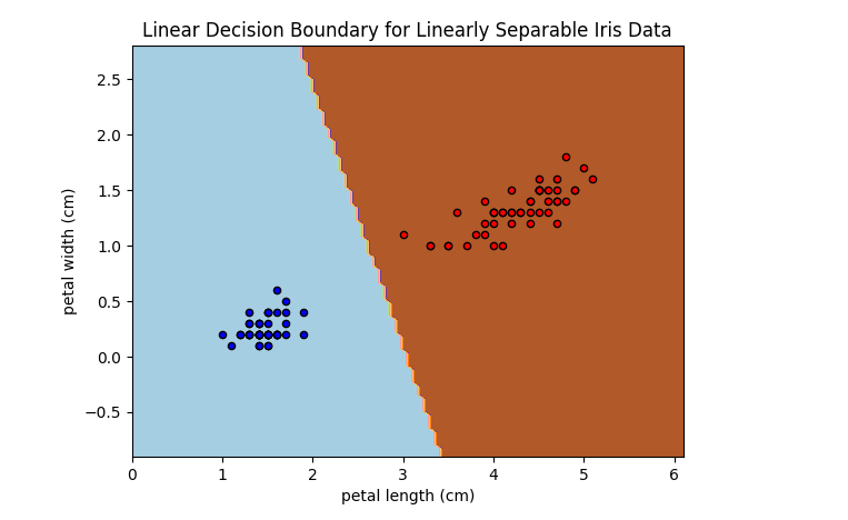
Resulting plot of the linear decision boundary for the Iris dataset.

Training on the Full Dataset

Let’s go back and train on the full dataset with all of the features.

How should we modify the code above? Implement the following high-level steps:

1. Create X and y variables pointing to your independent and dependent variables, respectively.

2. Split the data into training and test.

3. Train the model

4. Check the accuracy on the training and test data.

How does the accuracy compare with the previous version?

Solution:

>>> # We want to use the entire dataset, so we set X and y differently:
>>> X = iris.data
>>> y = iris.target

>>> # The rest is the same:
>>> # first, we split the data
>>> X_train, X_test, y_train, y_test = train_test_split(X, y, test_size=0.3, stratify=y, random_state=1)
>>> # next we
>>> clf = SGDClassifier(loss="perceptron", alpha=0.01)
>>> clf.fit(X_train, y_train)

>>> # Check the accuracy on the test data
>>> accuracy_test=accuracy_score(y_test, clf.predict(X_test))
>>> # Check accuracy on the training data
>>> accuracy_train=accuracy_score(y_train, clf.predict(X_train))
>>> print(f"Train accuracy: {accuracy_train}; Test accuracy: {accuracy_test}")

Visualizing the Confusion Matrix

A confusion matrix is a useful tool for understanding the performance of a model beyond just the accuracy rate.

A confusion matrix compares the predicated label of a model against the actual label for all values in the target class. It can be used to quickly target specific classes that the model might be performing better or worse on.

We can use the ConfusionMatrixDisplay.from_estimator() function to easily plot a confusion matrix for a model we have fit. See the sample code below:

>>> from sklearn.metrics import ConfusionMatrixDisplay
>>> cm_display = ConfusionMatrixDisplay.from_estimator(clf, X_test, y_test, cmap=plt.cm.Blues, normalize=None)

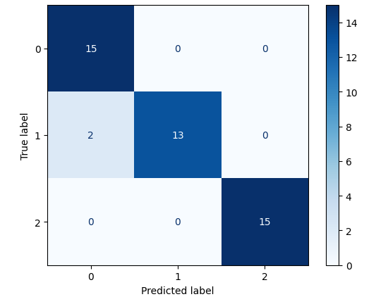
The confusion matrix above shows that our model did well predicting the Setosa (label 0) and the Virginica (label 2) flower types, but “confused” the Versicolor (label 1) for the Setosa two times.

Additional Resources

• Adapted from: COE 379L: Software Design For Responsible Intelligent Systems

• UC Berkeley CS189/289A: Introduction to Machine Learning.

• Numpy documentation

• SciKit-Learn train_test_split documentation

• SciKit-Learn iris dataset

• SciKit-Learn breast cancer dataset

References

[1]

Professor’s perceptron paved the way for AI - 60 years too soon. (2019). Cornell Chronicle

[2]

R. A. Fisher (1936). “The use of multiple measurements in taxonomic problems”. Annals of Eugenics. 7 (2): 179-188.