Exploratory Data Analysis with Jupyter Notebooks

The success of any data science project relies heavily on the quality and understanding of the data being analyzed. This includes things like training data for machine learning models, but also applies to any kind of data-driven analysis. An important first step is to familiarize yourself with the dataset you will be working with. This is a process called exploratory data analysis (EDA). We will mostly be using Python and the pandas library for this process. We will perform these steps in a Jupyter Notebook to show you how convenient it is for interactive data analysis and visualization.

By the end of this section, you should be able to:

• Load structured datasets into a pandas DataFrame

• Inspect and summarize data using .info(), .head(), and value counts

• Identify and handle missing values

• Drop or filter columns and rows based on criteria

• Convert string-based columns (e.g., age, dates) into numeric or datetime types

• Extract and manipulate date-related features (e.g., weekday, year)

• Visualize distributions using box plots, histograms, and scatter plots

• Compare patterns across subgroups (e.g., years, outcome types)

Start up a Jupyter Notebook and Install Dependencies

Before we can start exploring the data, we need to start up a Jupyter Notebook and make sure we have the necessary libraries installed. In this unit, we will be using pandas for data manipulation and seaborn and matplotlib for visualization.

[mbs337-vm]$ cd $HOME/mbs-337
[mbs337-vm]$ source .venv/bin/activate
(.venv) [mbs337-vm]$ curl ip.me
129.114.38.51
(.venv) [mbs337-vm]$ jupyter lab  # or "jupyter notebook"
[I 2026-03-01 17:40:03.353 ServerApp] jupyter_lsp | extension was successfully linked.
[I 2026-03-01 17:40:03.357 ServerApp] jupyter_server_terminals | extension was successfully linked.
[I 2026-03-01 17:40:03.361 ServerApp] jupyterlab | extension was successfully linked.
[I 2026-03-01 17:40:03.365 ServerApp] notebook | extension was successfully linked.
[I 2026-03-01 17:40:03.609 ServerApp] notebook_shim | extension was successfully linked.
[I 2026-03-01 17:40:03.623 ServerApp] notebook_shim | extension was successfully loaded.
[I 2026-03-01 17:40:03.625 ServerApp] jupyter_lsp | extension was successfully loaded.
[I 2026-03-01 17:40:03.626 ServerApp] jupyter_server_terminals | extension was successfully loaded.
[I 2026-03-01 17:40:03.628 LabApp] JupyterLab extension loaded from /home/ubuntu/mbs-337/.venv/lib/python3.12/site-packages/jupyterlab
[I 2026-03-01 17:40:03.628 LabApp] JupyterLab application directory is /home/ubuntu/mbs-337/.venv/share/jupyter/lab
[I 2026-03-01 17:40:03.628 LabApp] Extension Manager is 'pypi'.
[I 2026-03-01 17:40:03.670 ServerApp] jupyterlab | extension was successfully loaded.
[I 2026-03-01 17:40:03.673 ServerApp] notebook | extension was successfully loaded.
[I 2026-03-01 17:40:03.673 ServerApp] Serving notebooks from local directory: /home/ubuntu/mbs-337
[I 2026-03-01 17:40:03.673 ServerApp] Jupyter Server 2.17.0 is running at:
[I 2026-03-01 17:40:03.673 ServerApp] http://mbs-337-15:8888/lab
[I 2026-03-01 17:40:03.673 ServerApp]     http://127.0.0.1:8888/lab
[I 2026-03-01 17:40:03.674 ServerApp] Use Control-C to stop this server and shut down all kernels (twice to skip confirmation).

Go to a browser and enter the following URL to access the Jupyter Notebook/Lab interface using the public IP address of your Linux VM (that you got from the curl ip.me command above):

http://<your-vm-public-ip>:8888/lab  # or "http://<your-vm-public-ip>:8888/tree" for the classic notebook interface

Let’s install the necessary libraries from the notebook itself using pip:

!pip3 install pandas seaborn matplotlib

And make sure they’re installed by listing them:

!pip3 list

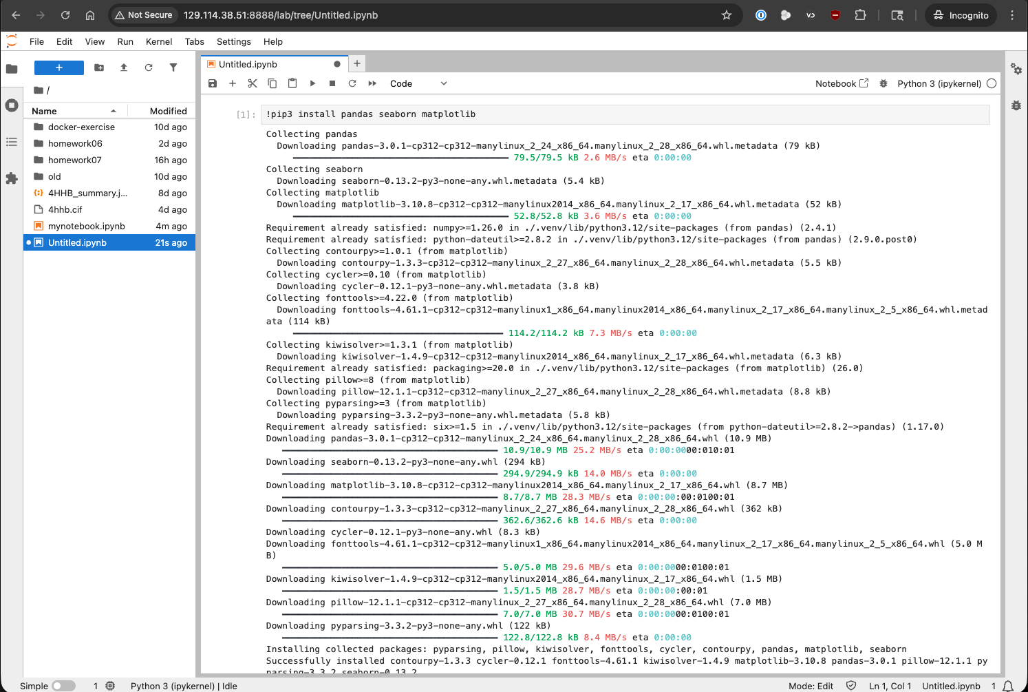
Pip installing directly from a Jupyter notebook cell.

Getting and Displaying the Data

We will be using a dataset from the City of Austin’s Open Data Portal, which contains publicly accessible datasets from the City’s data. Specifically, we’ll be using a dataset from the Austin Animal Center which tracks outcomes (status of animals as they leave the Center) which contains data from 10/01/2013 to 05/05/2025. This dataset includes information about the type of animal, its age, name, the outcome (e.g., adopted, transferred), and other relevant details. Before starting, you’ll need to load the this dataset into your Jupyter Notebook. It will be used throughout this section.

Instead of downloading and unzipping the file manually, we can now programmatically fetch and extract the data directly from the URL using Python. This approach makes your code more portable and reproducible.

>>> import requests
>>> import zipfile
>>> import io
>>> import pandas as pd

>>> # URL pointing to the ZIP file containing the CSV dataset
>>> url = 'https://raw.githubusercontent.com/tacc/mbs-337-sp26/main/docs/unit07/sample-data/Austin_Animal_Center_Outcomes.zip'

>>> # Send an HTTP GET request to fetch the content of the ZIP file
>>> response = requests.get(url)
>>> print(response.status_code)  # Should return 200 if the request was successful

>>> # Extract the ZIP file directly from the response's binary content
>>> with zipfile.ZipFile(io.BytesIO(response.content)) as z:

>>>     # Open the CSV file inside the ZIP without saving it to disk
>>>     with z.open('Austin_Animal_Center_Outcomes.csv') as csv_file:

>>>         # Read the CSV into a pandas DataFrame
>>>         data = pd.read_csv(csv_file)

>>>         # Display the first few rows of the DataFrame
>>>         display(data)

Explanation of the Code:

• requests.get(url): Sends an HTTP GET request to the specified URL to retrieve the content of the ZIP file.

• io.BytesIO(response.content): Creates an in-memory binary stream from the downloaded content, allowing it to be treated as a file-like object.

• zipfile.ZipFile(…): Opens the ZIP file from the in-memory binary stream.

• z.open(‘Austin_Animal_Center_Outcomes.csv’): Accesses the specific CSV file within the ZIP archive.

• pd.read_csv(csv_file): Reads the CSV file into a pandas DataFrame for data manipulation and analysis.

• display(data): Displays the DataFrame in a readable format, typically used in Jupyter notebooks.

This method avoids the need for manual downloading or unzipping and ensures your code can be run from any location with internet access.

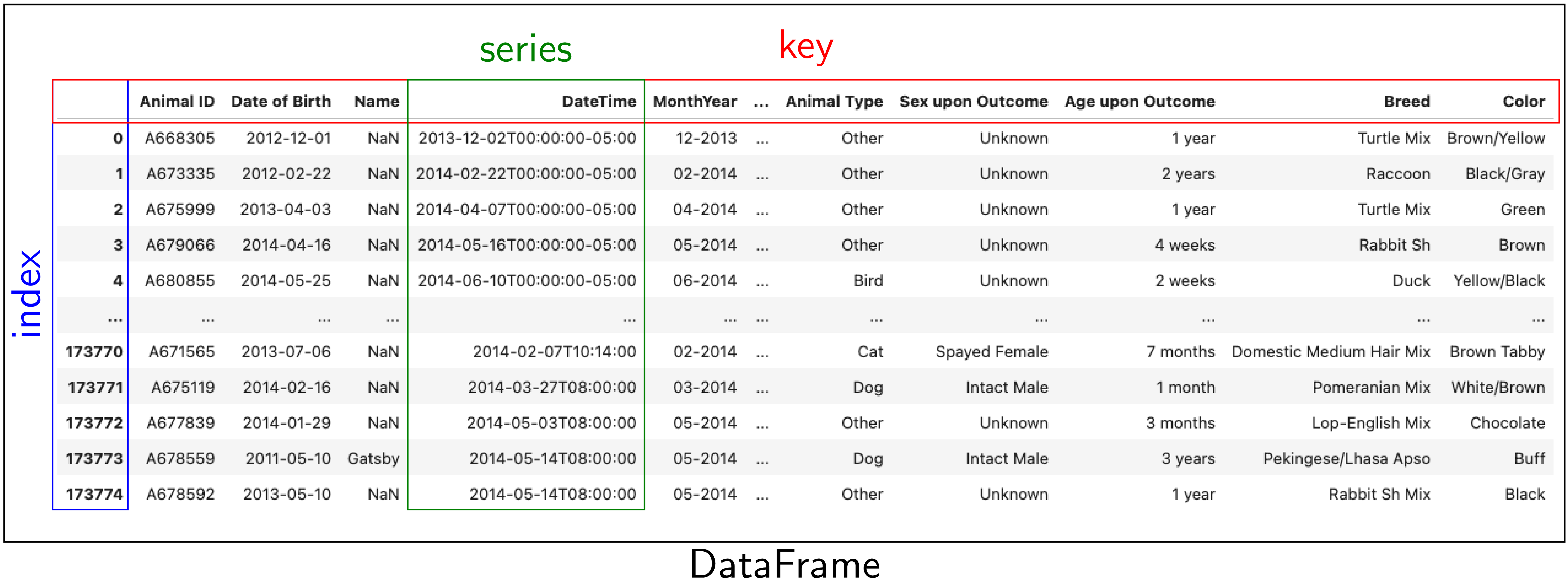
The image above represents a DataFrame, which is a 2D labeled data structure in pandas. Each column is a Series, each row is indexed (blue box), and column headers serve as keys (red box).

• index: row labels (blue)

• series: column of values (green)

• key: column name (red)

Note

Alternative method: You can also download the file manually using the link below, unzip it, and place Austin_Animal_Center_Outcomes.csv in your working directory.

• Austin_Animal_Center_Outcomes.zip

Once unzipped, make sure the CSV file is accessible from the notebook’s current folder, then you can load it using:

>>> import pandas as pd
>>> data = pd.read_csv('Austin_Animal_Center_Outcomes.csv')
>>> display(data)

Understanding the Structure

Once loaded, we can inspect the dataset. The first few rows give us a general sense of what we are working with.

Note

Commands preceded by >>> are meant to be run in a Python console or Jupyter notebook.

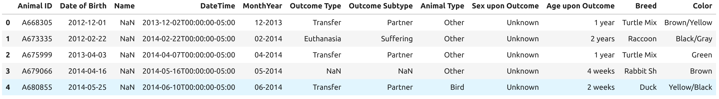
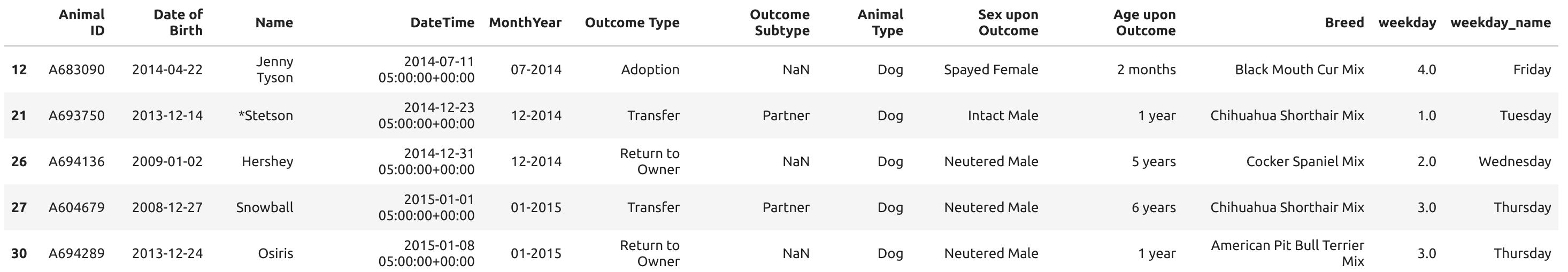
>>> data.head()

For more comprehensive info — like the total number of entries, data types, and missing values, we use .info():

>>> data.info()

<class 'pandas.core.frame.DataFrame'>
RangeIndex: 173775 entries, 0 to 173774
Data columns (total 12 columns):
 #   Column            Non-Null Count   Dtype
---  ------            --------------   -----
 0   Animal ID         173775 non-null  object
 1   Date of Birth     173775 non-null  object
 2   Name              123991 non-null  object
 3   DateTime          173775 non-null  object
 4   MonthYear         173775 non-null  object
 5   Outcome Type      173729 non-null  object
 6   Outcome Subtype   79660 non-null   object
 7   Animal Type       173775 non-null  object
 8   Sex upon Outcome  173774 non-null  object
 9   Age upon Outcome  173766 non-null  object
 10  Breed             173775 non-null  object
 11  Color             173775 non-null  object

We see that there are 173,775 records. Several fields (like Name and Outcome Subtype) contain missing values. All columns are currently stored as strings (object), even dates and age.

Dropping Unnecessary Columns

To streamline our analysis, we can drop columns that are not useful at this stage. For example, we won’t use the color of the animal in our initial exploration.

>>> data = data.drop(columns=['Color'], errors='ignore')
>>> data.info()

<class 'pandas.core.frame.DataFrame'>
RangeIndex: 173775 entries, 0 to 173774
Data columns (total 11 columns):
 #   Column            Non-Null Count   Dtype
---  ------            --------------   -----
 0   Animal ID         173775 non-null  object
 1   Date of Birth     173775 non-null  object
 2   Name              123991 non-null  object
 3   DateTime          173775 non-null  object
 4   MonthYear         173775 non-null  object
 5   Outcome Type      173729 non-null  object
 6   Outcome Subtype   79660 non-null   object
 7   Animal Type       173775 non-null  object
 8   Sex upon Outcome  173774 non-null  object
 9   Age upon Outcome  173766 non-null  object
 10  Breed             173775 non-null  object
dtypes: object(11)
memory usage: 14.6+ MB

Examining Columns and Values

We can list all columns in the dataset to better understand its structure:

>>> data.keys()

Index(['Animal ID', 'Date of Birth', 'Name', 'DateTime', 'MonthYear',
       'Outcome Type', 'Outcome Subtype', 'Animal Type', 'Sex upon Outcome',
       'Age upon Outcome', 'Breed'],
       dtype='object')

Let’s take a closer look at the Animal Type column:

>>> data['Animal Type']

0         Other
1         Other
2         Other
3         Other
4          Bird
          ...
173770      Cat
173771      Dog
173772    Other
173773      Dog
173774    Other
Name: Animal Type, Length: 173775, dtype: object

This column represents the type of animal (e.g., dog, cat, bird). We can get the unique types:

>>> data['Animal Type'].unique()

array(['Other', 'Bird', 'Dog', 'Cat', 'Livestock'], dtype=object)

And count how many records belong to each category:

>>> data['Animal Type'].value_counts()

Dog          94505
Cat          69399
Other         8960
Bird           877
Livestock       34

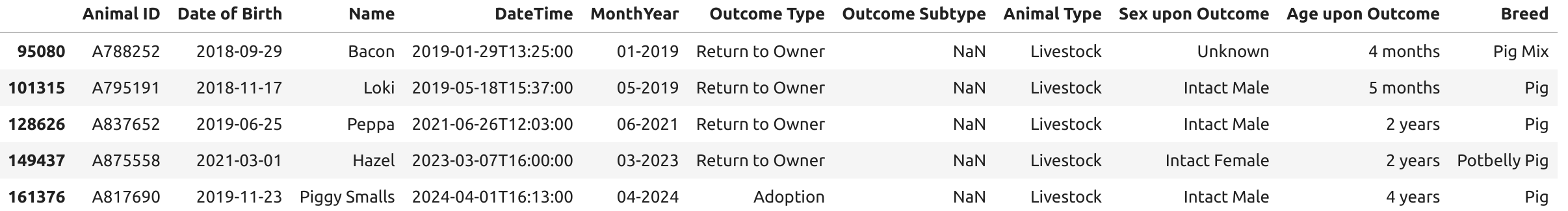
Finding All Livestock with Names

Let’s work on a real-world question: which livestock animals have names recorded in the system?

To answer this, we’ll walk through two essential data preparation steps:

• First, we’ll filter the dataset to isolate livestock records.

• Then, we’ll handle missing values by removing entries without names.

These steps reflect a common pattern in exploratory data analysis: narrowing the data to a relevant subgroup, then cleaning it to ensure quality before drawing any conclusions.

Filtering for Livestock

Our first step is to extract only the records where the animal type is 'Livestock'. We start by creating a Boolean mask that identifies rows where the 'Animal Type' column is equal to 'Livestock'. We then apply this filter to create a new DataFrame containing only those rows.

>>> filter_livestock = data['Animal Type'] == 'Livestock'
>>> data_livestock = data[filter_livestock]
>>> data_livestock.head()

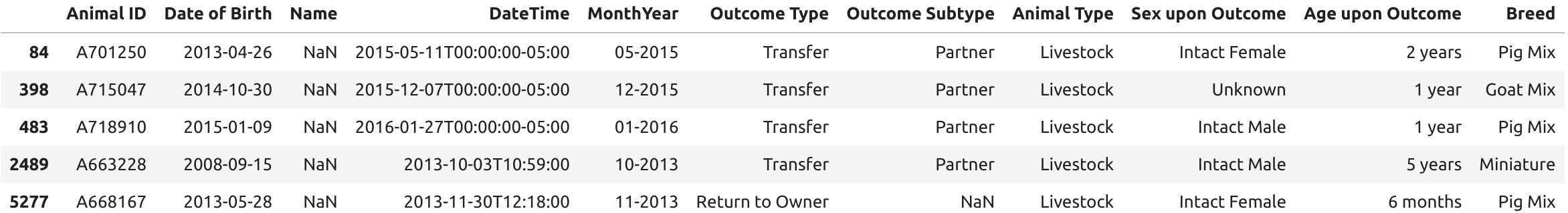
This filtered DataFrame contains only livestock records. From the preview, we can already see that some entries are missing values in the Name column.

Exercise: List All Livestock Names

Try listing all unique livestock names:

>>> data_livestock['Name'].unique()

array([nan, 'Bacon', 'Loki', 'Peppa', 'Hazel', 'Piggy Smalls'], dtype=object)

We can see that some livestock entries are missing a name (NaN). In most data analysis workflows, missing values like these need to be handled, either by imputing values or, as we’ll do here, removing incomplete rows.

Handling Missing Names

Next, we want to remove livestock entries without names. In practice, missing values are often removed or imputed depending on the context. Here, we’ll simply drop rows where the ``Name``` is missing.

We use the dropna() function, specifying the subset argument to limit the removal to rows where 'Name' is NaN.

>>> data_livestock = data_livestock.dropna(subset=['Name'])
>>> display(data_livestock)

This gives us a clean dataset of livestock animals that all have names recorded.

You’ve now completed a full data filtering and cleaning cycle.

Analyzing Dogs in the Dataset

Now let’s turn our attention to dogs, which make up the largest portion of the dataset. We’ll go through a few real-world data analysis steps to answer the following questions:

1. What is the oldest recorded dog in the dataset?

2. Can we extract and convert age information into numeric values for further analysis?

3. What can we learn by visualizing outcomes and age distribution for dogs?

Exercise: Find the Oldest Dog

Your first task is to create a new DataFrame, data_dog, that contains only dog entries with names recorded. Then, search for the oldest dog based on the 'Age upon Outcome' column.

>>> # Filter for dogs
>>> dog_filter = data['Animal Type'] == 'Dog'
>>> data_dog = data[dog_filter]

>>> # Remove unnamed entries
>>> data_dog = data_dog.dropna(subset=['Name'])

>>> # Preview unique age values
>>> print(data_dog['Age upon Outcome'].unique())

>>> # Filter and display dog(s) labeled as 24 years old
>>> filter_age = data_dog['Age upon Outcome'] == '24 years'
>>> display(data_dog[filter_age])

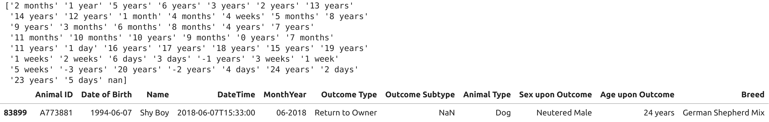
This exercise demonstrates how to create a filtered subset, clean it, and search for specific conditions in real data, a key part of exploratory data analysis.

Type Conversion

The 'Age upon Outcome' column is currently stored as a string (e.g., '3 years', '2 months'), which means we can’t perform numerical analysis directly on it. In this step, we will convert this string-based column into a proper numeric format so we can, for example, find the oldest dogs by age.

We will take the following steps:

1. Drop rows with missing age values. These entries can’t be processed numerically, so we remove them.

2. Filter rows that express age in years. We’ll ignore entries like ‘4 months’ or ‘2 weeks’ for now to simplify conversion.

3. Extract the numeric part of the string. We use a regular expression to extract just the digits (e.g., '4 years' → 4).

4. Convert the result to integers. This gives us a numeric AgeInYears column that we can use for filtering and visualization.

5. Find and display the oldest dogs. Now that we have numeric ages, we can identify and display the oldest dogs.

>>> # Remove rows where age is missing
>>> data_dog = data_dog.dropna(subset=['Age upon Outcome'])

>>> # Keep only rows where the age is expressed in full years
>>> years_filter = data_dog['Age upon Outcome'].str.contains('years')
>>> data_dog = data_dog[years_filter]

>>> # Extract the number of years from the string and convert to integer
>>> data_dog['AgeInYears'] = data_dog['Age upon Outcome'].str.extract(r'(\d+)')[0].astype(int)

>>> # Get the maximum age
>>> max_age = data_dog['AgeInYears'].max()
>>> print(f'The oldest dog is {max_age} years old.')

>>> # Display the record(s) corresponding to the oldest dog(s)
>>> display(data_dog[data_dog['AgeInYears'] == max_age])

This process is a good example of how to transform human-readable strings into numeric values that can be used for meaningful analysis.

Let’s take a closer look at this line:

data_dog['AgeInYears'] = data_dog['Age upon Outcome'].str.extract(r'(\d+)')[0].astype(int)

This command performs three important operations in a single step:

1. Accessing a string method on a pandas Series. The column ‘Age upon Outcome’ contains strings like '2 years', '14 years', etc. We use .str.extract() to apply a regular expression to each string in the Series.

2. Using a regular expression. The pattern r'(\d+)' means:

   • \d = match a digit (0-9)

   • + = one or more digits

   • parentheses () = capture the matched part so it becomes part of the output

   This extracts just the numeric portion from strings like '14 years', returning a new column with values like '14'.

3. Selecting the first capture group and converting to integer. The result of .str.extract() is a DataFrame (because there could be multiple groups). We use [0] to select the first column of matches.

   Then, .astype(int) converts the result from string (e.g., '14') to integer (14), allowing us to perform numeric operations.

The result is a new column called 'AgeInYears' that contains only numeric ages, ready for plotting or filtering.

Tip

If you’re unfamiliar with regular expressions, think of .str.extract(r'(\d+)') as a way to pull the number out of a string that looks like "14 years" — it’s like a smarter version of .split() or .replace().

Visualize Data

After performing type conversion and filtering, we can begin visualizing the data to understand trends and distributions. Visualization is a key part of exploratory data analysis, helping to reveal patterns that might not be obvious from raw numbers alone.

Box Plot of Dog Ages

We use a box plot to summarize the distribution of dog ages in years. This shows the median, quartiles, and outliers.

>>> import seaborn as sns
>>> import matplotlib.pyplot as plt
>>> sns.boxplot(data=data_dog, x='AgeInYears')

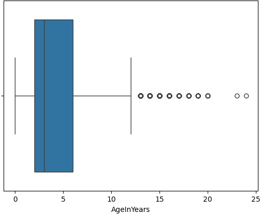
From this plot, we can quickly identify typical age ranges and see if any unusually young or old dogs are present.

Warning

Make sure to pip install any necessary dependencies!

Bar Plot of Outcome Types

We now look at what happens to the dogs. Were they adopted, transferred, returned, or something else? The 'Outcome Type' column records this.

>>> sns.histplot(data = data_dog['Outcome Type'])
>>> plt.xticks(rotation=45, ha='right')

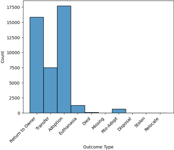
This bar chart shows the frequency of each outcome type. Rotating the x-axis labels makes them easier to read.

Exercise: Plot and Find the Most Common Outcome Subtype

Each outcome type can be broken down further. For example, a “Transfer” might go to a foster home, a partner shelter, or another facility. This detail is captured in the 'Outcome Subtype' column.

Try plotting the distribution of outcome subtypes to see which are most frequent.

>>> sns.histplot(data = data_dog['Outcome Subtype'])
>>> plt.xticks(rotation=45, ha='right')

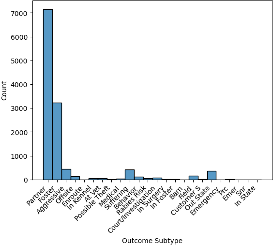
This visualization gives you more context about how different outcomes occur, for instance, whether transfers usually go to partners or other locations.

Working with Dates

Many datasets include timestamp information, which can be incredibly useful for time-based analysis. In our case, the 'DateTime' column records when each outcome occurred, but it is currently stored as a string, which limits what we can do with it.

To perform operations like grouping by day of the week, we first need to convert the column to a proper datetime object using pandas.

We then extract:

• The weekday number (0 = Monday, 6 = Sunday)

• The weekday name (e.g., ‘Monday’, ‘Tuesday’)

>>> # reset the data_dog DataFrame to include all dogs (not just those with ages)
>>> data_dog = data[dog_filter]

>>> # Convert the string to datetime, setting format='mixed' to safely handle different formats
>>> data_dog['DateTime'] = pd.to_datetime(data_dog['DateTime'], utc=True, format='mixed')
>>> data_dog.head()
>>> data_dog.info()

>>> # Extract the weekday number (0 = Monday, 6 = Sunday)
>>> data_dog['weekday'] = data_dog['DateTime'].dt.weekday

>>> # Extract the full weekday name (e.g., 'Monday', 'Tuesday')
>>> data_dog['weekday_name'] = data_dog['DateTime'].dt.day_name()

>>> # Preview the updated DataFrame
>>> data_dog.info()
>>> data_dog.head()

Now each dog outcome is labeled with the day of the week it occurred, both numerically and by name. This opens up the possibility of analyzing weekly patterns, for example, determining which day sees the most adoptions or the fewest returns.

Exercise: Which Day Has the Most and Least Outcomes?

>>> data_dog['weekday_name'].value_counts()

weekday_name
Tuesday      14701
Saturday     14025
Monday       13933
Friday       13740
Wednesday    12988
Thursday     12757
Sunday       12361
Name: count, dtype: int64

From the result, we can see that Tuesdays had the most outcomes, while Sundays had the fewest in this filtered dataset. This kind of temporal insight is often valuable when planning staffing or outreach for shelters.

Calculating the Overall Date Range

Now that we’ve converted the 'DateTime' column to proper datetime objects, we can calculate how long a time period the dataset covers.

This is helpful for understanding how recent the data is, and whether it spans days, months, or years, which can influence how you interpret trends over time.

>>> min_date = data_dog['DateTime'].min()
>>> max_date = data_dog['DateTime'].max()
>>> range_date = max_date - min_date
>>> print(range_date)

This code calculates:

• min_date: the earliest date in the dataset

• max_date: the most recent date

• range_date: the total time span between them

The result might look like:

4233 days 07:05:00

This tells us the filtered dataset covers approximately 10.3 years of outcomes for dogs.

Comparing Weekday Distributions for 2023 vs 2024

A useful exploratory question is: Did outcome patterns shift between years? To investigate this, we compare the distribution of dog outcomes by weekday in two different years: 2023 and 2024.

>>> # Filter the dataset by year
>>> data_2024 = data_dog[data_dog['DateTime'].dt.year == 2024]
>>> data_2023 = data_dog[data_dog['DateTime'].dt.year == 2023]

>>> # Count outcomes per weekday (0 = Monday, ..., 6 = Sunday)
>>> w2023 = data_2023['weekday'].value_counts().sort_index()
>>> w2024 = data_2024['weekday'].value_counts().sort_index()

This gives us the number of outcomes that occurred on each weekday, separately for each year.

Next, we plot the results:

>>> plt.figure(figsize=(8, 5))
>>> sns.scatterplot(x=w2023.index, y=w2023.values, label='2023')
>>> sns.scatterplot(x=w2024.index, y=w2024.values, label='2024')
>>> plt.xticks(ticks=range(7), labels=['Mon', 'Tue', 'Wed', 'Thu', 'Fri', 'Sat', 'Sun'])
>>> plt.title('Dog Outcomes by Weekday: 2023 vs 2024')
>>> plt.xlabel('Weekday')
>>> plt.ylabel('Number of Outcomes')
>>> plt.legend()
>>> plt.grid(True)
>>> plt.show()

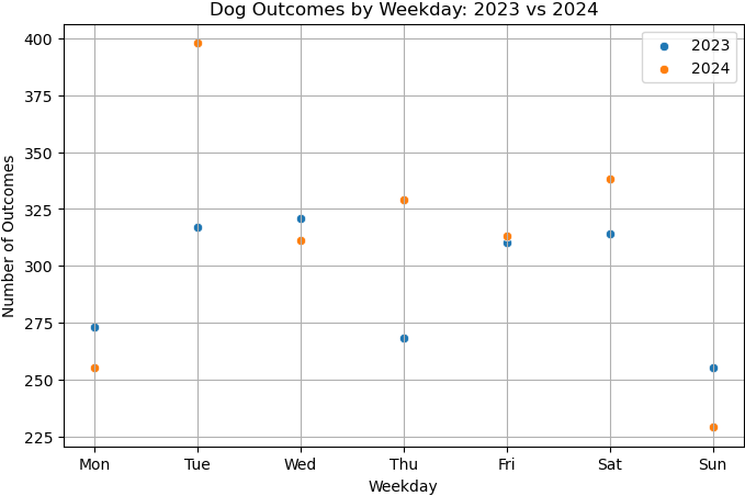
From this plot, you can visually compare the activity levels across the week between the two years. For example, if adoptions were much higher on Tuesdays and Thursdays in 2024 compared to 2023, that might signal a shift in shelter scheduling or public behavior.

Conclusion

You now know how to:

• Explore real datasets using pandas

• Visualize distributions with seaborn

• Clean and transform data for analysis

In a practical setting, you would typically perform these steps interactively on your own data prior to training a machine learning model. Once finished, going back through the steps and saving them to a new script is good practice. This way, you can reproduce your EDA process and share it with others.

Summary of Common EDA Operations

Here’s a reference table of the main operations and functions covered in this tutorial:

Step	Purpose	Common Function(s)
Load data	Import CSV as a DataFrame	pd.read_csv()
Preview data	Look at the first few rows	data.head(), display(data)
Inspect structure	Check types, memory usage, and missing values	data.info()
Column overview	See column names and value counts	data.keys(), data['col'].value_counts()
Handle missing data	Remove rows with NaN in specific columns	data.dropna(subset=['col'])
Filter rows	Create subsets based on condition	data[data['col'] == 'value']
Type conversion	Convert strings to numbers or dates	astype(int), pd.to_datetime()
Extract from strings	Parse numeric values from strings	.str.extract(r'(\\d+)'), .str.split()
Work with dates	Get weekday, year, etc.	.dt.weekday, .dt.day_name(), .dt.year
Summary statistics	Min, max, range of dates	data['Date'].min(), .max(), .max() - .min()
Visualize distributions	Understand data shape and outliers	sns.boxplot(), sns.histplot()
Compare groups	Examine trends across years or categories	value_counts(), scatterplot()

Additional Resources

• Pandas reference documentation

• Seaborn reference documentation

• Matplotlib reference documentation